Alternative to Multiple IF Statements
April 30, 2013
Have you ever had to create a multiple IF statement? Ever notice how crazy it looks with all those parentheses and it’s difficult to follow? Well, I was wondering if there was another way I could create a multiple IF statements that would be cleaner and easier to edit if need be.
And I have.
What I have discovered isn’t exactly as powerful as an IF statement, however, this does give you an alternative way to create a big IF statement if you need to match exact values.
Technically, I haven’t actually determined all the possibilities of this technique, but what I do know is that if you have a nested IF statement that does a basic 1-to-1 comparison, this is a pretty interesting and clean alternative than using a lot of IF statements.
Just to be clear:
So far, I found that this works best for exact matching in an IF statement
IF Statement the Regular Way
Here’s an example. Say you had the following requirements:
| Data | Desired Output |
|---|---|
| Yes | Definitely |
| No | Certainly Not |
| Maybe | Eh |
A pretty standard IF formula to take the data and transform it to the desired output would be:
=IF(A1="Yes","Definitely",IF(A1="No","Certainly Not",IF(A1="Maybe","Eh")))This works fine, but notice how A1 is repeated? What if you had to change that? You would have to change that in multiple places, which isn’t so bad for this particular case. However, have you ever had a complicated INDEX+MATCH function? Let’s look at another example. Say I have the data:
| Person | Response |
|---|---|
| Joseph | Yes |
| John | Maybe |
| Meredith | No |
| more names | more responses |
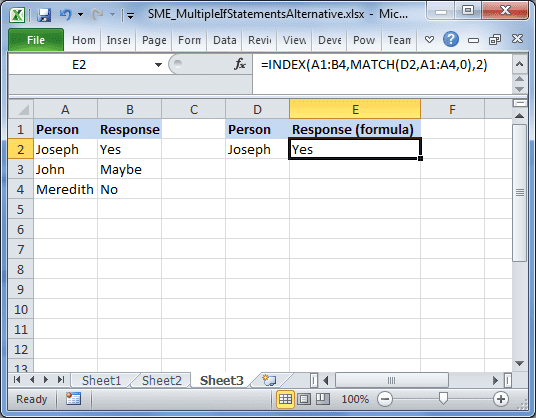
I want to look up a person’s response using an INDEX+MATCH function. I would use something like:
=INDEX($A$1:$B$4,MATCH(D2,$A$1:$A$4,0),2)Assuming that the desired lookup_value is in D2 like the image below:
Now I’d like to transform that “Yes” to “Definitely” and the other responses to “Certainly Not” and “Eh” as before. The formula would look like:
=IF(INDEX($A$1:$B$4, MATCH(D2,$A$1:$A$4,0),2)="Yes","Definitely", IF(INDEX($A$1:$B$4, MATCH(D2,$A$1:$A$4,0),2)="Maybe","Eh", IF(INDEX($A$1:$B$4, MATCH(D2,$A$1:$A$4,0),2)="No","Certainly Not")))Not so pretty. It’s a bit complicated and not so easy to follow if you look at the formula bar in Excel with this formula. Plus, if you have to change the INDEX formula, you have to change it in 3 spots (something that has always irked me - as a developer, you try to not repeat any code if you can help it).
So, how can I make this cleaner?
Alternative to Multiple IF Statements
This is a little unorthodox, but it’s pretty neat for something like this.
Use INDEX and MATCH with array constants to map the matching values to the desired results
If you’re not familiar with a array constants, it’s pretty simple. Using the curly braces { and }, you can create the array constants of data. In the case of the INDEX and MATCH functions, they actually accept array parameters, so you can either give it a Range (this is usually the case), or you can use these curly braces to create array constants. John Walkenbach wrote a nice piece on the subject. Please have a look if you would like more info.
Here’s the format:
=INDEX({desired results}, MATCH(lookup_value, {values to compare},0))| Item | Explanation |
|---|---|
| desired results | This would be the list of “Definitely,” “Certainly Not,” and “Eh” |
lookup_value |
Surprisingly, this would be the main INDEX+MATCH formula that we had to repeat in the multiple if statements earlier. Basically, this part of the formula is what will get evaluated, much like the first parameter in an IF statement. |
| values to compare | These would be the “Yes,” “No,” and “Maybe” list |
Putting this together we now have the following formula:
=INDEX({"Definitely","Certainly Not","Eh"},MATCH( INDEX($A$1:$B$4,MATCH(D2,$A$1:$A$4,0),2), {"Yes","No","Maybe"},0))I did say that it would be a little unorthodox :) but check it out! You only have to write the main INDEX+MATCH function one time, and you don’t have a bazillion parentheses. Awesome.
Now, I know that this is a very simple example, but it’s only to illustrate the point.
How this Works
In order to get this to work right, you have to follow 3 rules:
- The array constants
{"Definitely","Certainly Not","Eh"}must match the desired outputs array constants{"Yes","No","Maybe"}. Since “Definitely” is in the first spot, it matches to “Yes.” This is crucial to making sure you get the desired output correct. - The first parameter in MATCH must contain a value that is found in the INDEX array constant.
- You must wear cool sunglasses and eat a turkey sandwich
Well, ok, you only need the first 2 rules, but you get it :)
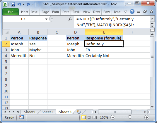
Let’s look at the function from E2 below:
The formula starts off with the INDEX function inside of the MATCH function. It finds “Joseph” and moves over one cell to find “Yes”
=INDEX({"Definitely","Certainly Not","Eh"},MATCH("Yes", {"Yes","No","Maybe"},0))The “Yes” matches with the first “Yes” in the array constant, and so it will return 1 because MATCH will return a row number of what it finds.
=INDEX({"Definitely","Certainly Not","Eh"},1)The row number 1 in the INDEX function will match up with the “Definitely” item in the array constant of INDEX, which will then return “Definitely”
="Definitely"This results in the desired result of “Definitely.”
Granted, you technically could use Ranges instead of the array constants, however, I wanted to illustrate it this way for two reasons:
- It’s a little simpler this way both in teaching and in practice
- I don’t always agree with creating an entire worksheet just to hold a simple list like this
However, if these lists were very big, then I would encourage maintaining named ranges for them so the formulas are much cleaner.
Well, that’s it. I hope you found this info unique and interesting :) Until we meet again!


