Array Formulas for Beginners

Excel Array formulas are one of the handiest tools to have under your Excel tool belt. You can expand regular Excel formulas to provide a lot more power to regular functions. Take the function AVERAGEIF() as an example.

Before Excel 2007, you had to use array formulas to provide the same functionality. And while array formulas are extremely powerful, they can also be one of the most confusing features of Excel to learn.

So, in this post, let’s learn how to use Excel array formulas as easy as possible.

There is so much you can learn with array formulas in Excel that I could probably write an essay on the subject. However, for the sake of brevity, this will be a simple introduction to arrays to get you familiar with the concept.

What’s an array?

Some people reading this might not be sure what an array is. Basically, an array in Excel is typically a simple set of data. This data can be text, numbers, or both. It’s very similar to a list. If I were to ask you what you needed to buy from the grocery store, you might give me this list:

• Milk
• Eggs
• Paper Towels
• Sandwich Bags

Put into an Excel array format, it would look like:

{"Milk";"Eggs";"Paper Towels";"Sandwich Bags"}

The curly braces {...} denotes the set of data (in other words, the array itself). Each item in the “list” is separated by a semi-colon. For text items, they are encapsulated with quotations, like in the example above. Arrays can be a mixture of different data types like text and numbers in one array. The idea to remember is that an array is a list that you can put any type of data into.

Array formulas in Excel are entered by creating the formula like normal (begin with the equal sign, etc.), but instead of pressing Enter, you press Ctrl+Shift+Enter (press and hold Ctrl, press and hold Shift, then press Enter and let go of all three). After we finish entering the formula with Ctrl+Shift+Enter, the formula will be surrounded by curly braces {=...} as in the following example:

{=AVERAGE(IF($A$2:$A$10>20,$A$2:$A$10))}

Please note that you can’t actually type the curly braces into an Excel formula and have it become an array formula. You need to type Ctrl+Shift+Enter when editing the formula.

I would like to mention at this point that this example of a single-dimension array. We’ll cover multi-dimension arrays in another post.

Does this article help you? If so, please consider supporting me with a coffee ☕️

So, what are array formulas?

The array by itself isn’t particularly useful. When you put them in conjunction with Excel functions is when you harness the true power of array formulas. Let’s start with a simple example.

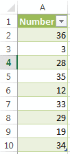
If I were to take the average of these numbers, I get 25.44 (repeating, of course). Let’s add the condition that I only want to average those numbers that are greater than 20. To build the formula, I need to first grab all of the numbers that are greater than 20 (create an array of them), and then average those numbers.

We’re going to use theIF() function to return the list of numbers greater than 20. Here’s what this part of the formula looks like:

=AVERAGE(IF($A$2:$A$10>20,$A$2:$A$10))
         ----------------------------

When this formula is entered as an array formula (using Ctrl+Shift+Enter), it will take each argument and convert it into an array and process each element in all arrays like so:

=AVERAGE(
    IF(
    {36; 3; 28; 35; 12; 33; 29; 19; 34}>20,
    {36; 3; 28; 35; 12; 33; 29; 19; 34},
    )
)

The first argument is the condition. Excel will look at each element in the first array and check if it is greater than 20. If so, it will evaluate to TRUE, otherwise it will evaluate to FALSE. Take a look at the first value of 36:

=AVERAGE(
    IF(
    { 36 > 20; 3; 28; 35; 12; 33; 29; 19; 34},
      -------
    { 36;      3; 28; 35; 12; 33; 29; 19; 34}
    )
)

The underlined section 36 > 20 will evaluate to TRUE. When it is done checking all the conditions, it will create a new array of TRUE/FALSE for each element it checked and replace the old array with the TRUE/FALSE array like so:

=AVERAGE(
    IF(
    { TRUE; FALSE; TRUE; TRUE; FALSE; TRUE; TRUE; FALSE; TRUE},
    {   36;     3;   28;   35;    12;   33;   29;    19;   34}
    )
)

Now the formula will match up those items which are true and return the corresponding number and return only those numbers that match up with TRUE:

=AVERAGE(
    IF(
    { TRUE; FALSE; TRUE; TRUE; FALSE; TRUE; TRUE; FALSE; TRUE},
      -----        ----- -----        ----- -----        ----
    {   36;     3;   28;   35;    12;   33;   29;    19;   34}
        ---          ---   ---          ---   ---          --
    )
)

Becomes:

=AVERAGE({ 36; 28; 35; 33; 29; 34})
           --- --- --- --- --- --

Now the AVERAGE() function will work with averaging those numbers returned, which results in:

32.5

I hope this post helps you better understand how Excel works out an array formula. I’ll be posting more articles in the near future with more examples using array formulas. If you have any questions, feel free to comment below!