How to Split Cells in Excel

In my last post, we talked about how to join cells with a comma using VBA. This week, I’d like to discuss how to split cells in Excel. You might need to split one cell into multiple cells for a few reasons:

• You downloaded a file that Excel didn’t know how to split (log files can be an example of this).
• You have a column that you want to split into multiple columns based on a specific character.
• …ok, I know I said a “few reasons,” but I can only think of 2 reasons why you’d like to do this. However, I’m sure you have run into other reasons for needing this. If so, please share them with us in the comments!

So let’s dig in and see how we can split cells in Excel.

Split Cells in Excel

Most of the time, you will probably need to split cells in Excel without having to use any advanced feature. The typical case is when you have a set of cells that have info in them that should be broken up by a comma, semicolon, tab, or other character.

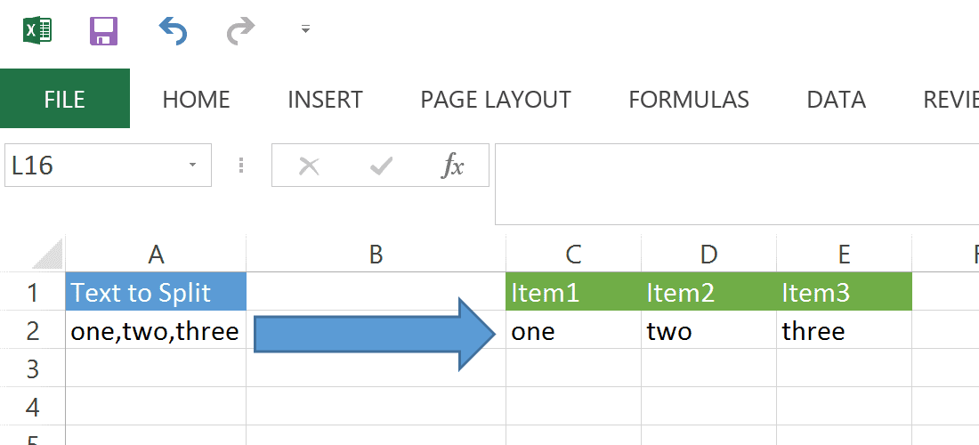
Say you have this simple set of data:

Here we have a single cell that has 3 items in them separated by a comma.

In Excel, there is a tool we’re going to use called Text to Columns. This tool will take a columns of cells and separate them into multiple adjacent cells based on a character that you specify.

Click in the Data tab —> Text to Columns

A Wizard will pop-up and help you split cells in Excel:

In this wizard, you will be guided on how to split up your cells into multiple ones. There are a lot of options you can choose from and it can get a little complicated, so let’s step through it.[/text_output][text_output]

Does this article help you? If so, please consider supporting me with a coffee ☕️

Step 1 - Fixed Width or Delimited

In the first window that pops up, you will be asked if your data has a fixed width or it is delimited.

Delimited

This is a very common choice. A delimited data set means that you have data that should be split up by some character - like a comma. In our example, we’re going to split up the data with a comma.

item one,item two,item three

Fixed Width

Fixed Width means that there is a certain amount of “white space” between each column in your data set. For example, if you have a Tab between each column, our example might look like this:

item one    item two    item three

In the text above, each item is separated by 4 spaces. Since each section between each item has the same amount of spaces, Excel will understand this to be the delimiter to split up the cell into multiple cells.

For our example, we will pick Delimited. Click Next.

Step 2 - Choose your Delimiter

The next step is to choose which character you want to split up the cell by. “Tab” is selected by default. In our example, let’s uncheck “Tab” and check “Comma” instead.

Selecting Multiple Delimiters

Notice that these are checkboxes and not radio buttons. This means that if you have multiple Delimiters selected, then the cell will be split up by as many delimiters as you specify in this list.

Check out the Data Preview section. The vertical lines indicate the new cells that will be created by splitting up the cell you selected. Click Next.

Step 3 - Formatting the new data

In the last step, this is where you format each column’s data. This part of the wizard has some interesting advanced settings, which we will get into in a later post. For now, we will accept the default settings. Click Finish.

Results

Once you hit finish, Excel will take the cell you selected and split it up into multiple columns based on how many commas it found in the cell. For this example, there were 2 commas, which resulted in 3 columns (since data was found on either side of each comma).

I know this was a very basic example of how to split cells in Excel, but I wanted to give you a quick intro on the tool that Excel provides. Do you have any specific questions on splitting up cells in Excel? Please let me know in the comments below! I’m curious to know what you’d like to learn about this feature for future posts.