Create a Unique List in Excel based on Criteria
February 23, 2017
Nathan is working on a spreadsheet that contains a list of car models and
owners. He needs to create a unique list of owners per car. “Maybe I can use an
IF() formula,” he thinks to himself and decides to give it a go. However,
after several failed attempts he decides to search the web to see how people
create a unique list in Excel based on a specific condition. He comes across a
formula that looks pretty complicated, but others had claimed it worked for
them, so Nathan decides to give it a whirl. Then he copy/pastes the formula in a
cell and adjusts the ranges for his worksheet. After that he copies the formula
down to create the list. It works! “Perfect,” Nathan excitedly thinks to
himself, “now I’ll just copy that to the right…” and when he does, the formula
breaks. He tries modifying the formula, but it’s too advanced for him. One small
change upsets the formula and returns errors. Frustrated and tired, he
reluctantly decides he’ll just create the list by hand.
Does this sound familiar? We’ve all been here at one point or another. The problem with these complicated formulas is that most people don’t understand what they’re copying / pasting into Excel. This leads to many tries and retries, only to lead to frustration. Excel has literally hundreds of formulas and it’s easy to get lost if you have a lot of nested functions to work with. It’s great that people share their clever formulas online and the internet is full of helpful advice, but if you find a formula online and simply copy / paste it without understanding how it works, you limit yourself from the power it has, and therefore, you limit the power that you have.
In this post, I’d like to walk us through how to understand one of these complicated formulas: how to create a unique list in Excel based on criteria. Let’s get started.
The Problem
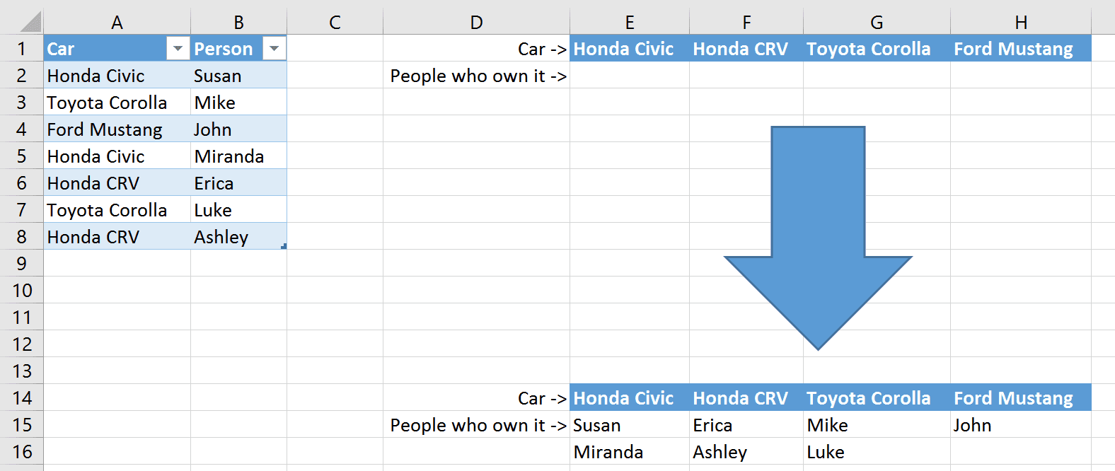
Let’s say you have this basic info:

Download this workbook to follow along.
On the left is an Excel Table named Cars (if you’re not familiar with Excel Tables, click here). This will be our data source we want to create a list from.
On the right side of the worksheet is where we will make that list, with each car in its own column. Note that there are duplicate cars owned by different people in the data source - this can make it difficult to create a unique list of car owners, which is why we need a more advanced formula.
We also want the formula needs to be dynamic, meaning that we can copy it down and to the right to create the unique lists for each car model.
How do you think you would construct this kind of formula?
Does this article help you? If so, please consider supporting me with a coffee ☕️
The Solution
Here’s what the resulting formula will look like:
=IFERROR(INDEX(Cars,SMALL(IF(Cars[Car]=E$1,ROW(Cars)-1),ROW(1:1)),2),"")Please note that this is an array formula and must be entered by
pressing Ctrl+Shift+Enter.
Click here to
learn more about array formulas.
When we enter this in E2, we get Susan as the first answer.

Then copy down and to the right and we have our solution:

Before You Simply Copy / Paste!
Remember what we discussed in the intro? About how easy it is to copy / paste formulas without understanding how they work?
How easy is it to copy / paste answers like these?
Very easy.
And how much power does doing that have?
Very little.
Don’t you want to harness the power of building complex formulas?

How does this formula work?
Let’s break this formula down piece-by-piece to understand what’s really going on.
First, the main IFERROR() function is there to handle any errors and replaces
them with a blank cell. Let’s now focus on the part of the formula that’s doing
the real work.
The Index() Function’s Role
The INDEX() formula works like so: INDEX(array, row, column)
Here is our INDEX() formula for the unique list we are trying to create:
INDEX(Cars,SMALL(IF(Cars[Car]=E$1,ROW(Cars)-1),ROW(1:1)),2)
        |__| |_________________________________________| |
         |                      |                        |
        array                  row                     column
If you’re not familiar with the INDEX() function, check out
this link
to learn more.
Basically, the INDEX() function will look at a table (the array), then based
on the ROW and COLUMN you give it, a single value will be returned. This
single value will be one of the items in our unique list. The secret here is to
manipulate the ROW portion, which we will dig into shortly.
The array that we reference is the Cars table.
The ROW portion of the formula has a more complicated formula which allows us
to get a list of non-repeating values from the data set. This is actually where
the
Array Formula
(Ctrl+Shift+Enter) is required and where the unique list comes from.
The COLUMN portion simply says 2, which means “use the 2nd column from the
array (table) I’ve given you.” While the 2nd column in our case is column B,
the formula actually refers to the 2nd column of the array you gave it. If we
had our table starting in cell E5, the 2nd column of the table would be in
column F.
The Small() Function’s Role
Let’s break down the ROW portion of the INDEX() function a bit further.
The SMALL() function simply says:
SMALL(data_set, k-th_smallest_item)Here is the formula:
SMALL(IF(Cars[Car]=E$1,ROW(Cars)-1),ROW(1:1))
      |___________________________| |______|
                  |                    |
              data_set         k-th_smallest_item
Here’s a quick sample formula to better understand how the SMALL() function works:
=SMALL({4,5,1,3}, 2)The data set is an array of 4, 5, 1, and 3. The k-th_smallest_item of the
formula is set to 2. This returns the second smallest item of the set, which
is 3.
Both portions of our SMALL() function have another formula in them. Let’s dig
into this even further (we’re almost there, I promise).
The If() Function’s Role in the data_set Portion
IF(Cars[Car]=E$1,ROW(Cars)-1)This is the part that needs the array formula (Ctrl+Shift+Enter) and this is
also where things get a little tricky, but it’s not as bad as you might think.
This function is looking in the Car column of the Cars table and looking for a
match from cell E1, which is the Car’s make and model. If True, we want to
return the row number of where that Car was found. We use the ROW() function
to accomplish that. Right now, we’re looking to find the owners of the Honda
Civic, which are Susan and Miranda. To get that, we first need to find all of
the rows that match the car that we’re looking for, then we will simply move 1
cell to the right to get the name of the owner. All matching rows of cars will
have the corresponding owners in the next cell and this is how we will get our
unique list.
A Note about the word ‘Rows’
I’d like to take a second and explain something about the word “Rows”.
When working with Excel Tables (or any “data array”) it’s important to realize that the first “row of data” is actually considered Row 1 regardless of whether the data starts at A1 or Z35. When using the
INDEX()function and your data is inC5:D10and you have headers inC5andD5, then your data begins atC6and ends atD10. Even though on the worksheet it’s the 6th row for where the data begins, it’s still considered Row1in yourINDEX()function (and other functions that work with arrays).Because of this confusion, I will refer to rows in an array as “data rows” and rows in the worksheet as “worksheet rows”.
The reason for the -1 is because if you take the Honda Civic as an example,
that text first appears on row 2 of the worksheet. While the Excel Table’s
data begins on Row 2, the first “row of data” is still considered “row 1” when
working with the table (these are data rows). The ROW() function only returns
rows of the worksheet, regardless of any data you may be referencing. And since
ROW() will return 2 for Honda Civic, we need to adjust for how INDEX()
is working with the data rows.
For finding Susan and Miranda, those would be data rows 1 and 4 because
the data starts in A2 and ends in B8.
Here’s how this IF() function is broken down:
IF(Cars[Car]=E$1,ROW(Cars)-1)Cars[Car] becomes:
IF({"Honda Civic";"Toyota Corolla";"Ford Mustang";"Honda Civic";"Honda CRV";"Toyota Corolla";"Honda CRV"}=E$1,ROW(Cars)-1)E$1 becomes:
IF({"Honda Civic";"Toyota Corolla";"Ford Mustang";"Honda Civic";"Honda CRV";"Toyota Corolla";"Honda CRV"}="Honda Civic",ROW(Cars)-1)
    -------------                                 -------------                                           -------------
Notice that I underlined the matches that will be made. This will
correspond to how the condition section is evaluated in the IF() function:
IF({TRUE;FALSE;FALSE;TRUE;FALSE;FALSE;FALSE},ROW(Cars)-1)
    ----             ----
Now, the ROW(Cars)-1 part gets evaluated:
IF({TRUE;FALSE;FALSE;TRUE;FALSE;FALSE;FALSE},{1;2;3;4;5;6;7})
    ----             ----                     -     -
Also, since we didn’t include a value_if_false section for the IF statement,
Excel gives us FALSE be default. The resulting IF formula is actually:
IF({TRUE;FALSE;FALSE;TRUE;FALSE;FALSE;FALSE},{1;2;3;4;5;6;7},{FALSE;FALSE;FALSE;FALSE;FALSE;FALSE;FALSE})The TRUE matches in the first parameter of the IF statement will correspond
to the same item in the value_if_true section, whereas if FALSE is found in
the IF statement, we simply get FALSE as the IF formula is building up the
resulting array. The resulting formula after the IF statement is evaluated is:
{1;FALSE;FALSE;4;FALSE;FALSE;FALSE}
 -             -
What this says is for the Honda Civic, we found Honda Civic in data rows 1 and 4
(which correspond to the data rows where Susan and Miranda are).
The Row() Function’s Role in the k-th_smallest_item Portion
Coming back to our SMALL() function:
SMALL({1;FALSE;FALSE;4;FALSE;FALSE;FALSE},ROW(1:1))The part:
ROW(1:1)Will simply return 1 when we put the formula in cell E2, like we are. When
we copy the formula down, it will become ROW(2:2) which will return 2.
Because this formula is sitting in the k-th_smallest_item portion of the
SMALL() function, when we copy the formula down, instead of using the first
match of who has a Honda Civic (i.e. Susan) we will use the 2nd owner (i.e.
Miranda).
SMALL({1;FALSE;FALSE;4;FALSE;FALSE;FALSE},1)This will now simply pick the 1st smallest item in the set, which is 1. Note
that it ignores the FALSE items in the set.
The result for the SMALL() function is simply:
1Putting it all back together
Coming back to the formula:
INDEX(Cars,SMALL(IF(Cars[Car]=E$1,ROW(Cars)-1),ROW(1:1)),2)When this is in cell E2, the evaluation is:
INDEX(Cars,1,2)Which means to say, “in the Cars table, return data row 1 and data column 2,”
corresponding to Susan. That’s what we get for the first formula.
When we copy the formula down by one cell (in E3), here is the breakdown (with
changes underlined):
INDEX(Cars,SMALL(IF(Cars[Car]=E$1,ROW(Cars)-1),ROW(2:2)),2)
                                               --------

INDEX(Cars,SMALL({1;FALSE;FALSE;4;FALSE;FALSE;FALSE},2)),2)
                                -                    -

INDEX(Cars,4,2)

Miranda
Notice here that since ROW(1:1) changed to ROW(2:2) that it’s simply
adjusting our k-th_smallest_item in the SMALL() function, which is how we
can avoid creating duplicates.
Also notice that when you copy to the right, the ONLY thing that changes is the
column in the IF() function:
INDEX(Cars,SMALL(IF(Cars[Car]=F$1,ROW(Cars)-1),ROW(1:1)),2)I didn’t lock this column so we can simply copy to the right and have the rest of the worksheet adapt correctly.
What happens if you copy down or to the right too far?
You’ll get a #NUM! error, which is why we put the IFERROR() portion in there
(to make any error just show a blank string…essentially hiding the errors).