How to Count Unique Values
September 27, 2017
If you ever needed a function in Excel called CountUnique(), you might be
disappointed to find that no such function exists in Excel. However, there’s a
simple trick that we can employ that will do the same thing: CountIf(). Let’s
take a look.
How to Count Unique Values using CountIf and Sum
Here is the formula we’ll be working with:
=SUM(1/COUNTIF(range,range))Where range is the same range, applied twice to the CountIf function.
Also, this is an array formula, and should be entered with Ctrl+Shift+Enter
(Cmd+Shift+Enter on Mac). To learn more about array formulas,
click here.
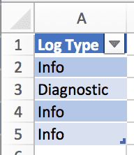
Let’s say that we have this simple table called Logs:
How can we count unique values using this formula? Here’s what the formula looks like:
{=SUM(1/COUNTIF(Logs[Log Type],Logs[Log Type]))}With a result of 2.
Notice that for the COUNTIF() function I repeat the same range. Also, if
you’re wondering about the syntax, please see my post about
Excel Tables and
Structured References.
How this Works
Let’s break this down piece-by-piece to understand what’s going on here.
Since this is an array function, the COUNTIF(range,range) portion looks
something like this:
First, evaluate the table reference to ranges:
COUNTIF(A2:A5,A2:A5)Next, evaluate the ranges to their values in an array format:
COUNTIF({"Info","Diagnostic","Info","Info"},{"Info","Diagnostic","Info","Info"})Note that the first parameter is the range being checked and the second parameter is the set of values that Excel will check for equality.
The first round will look something like this:
COUNTIF({"Info","Diagnostic","Info","Info"},{"Info","Diagnostic","Info","Info"})The first Info on the left was found 3 times on the right.
COUNTIF({"Info","Diagnostic","Info","Info"},{"Info","Diagnostic","Info","Info"})
          ----                                ----                ----   ----

Result:
COUNTIF({3,"Diagnostic","Info","Info"},{"Info","Diagnostic","Info","Info"})
         -
Then, Diagnotic was found 1 time on the right:
COUNTIF({3,"Diagnostic","Info","Info"},{"Info","Diagnostic","Info","Info"})
            ----------                          ----------

Result:
COUNTIF({3,1,"Info","Info"},{"Info","Diagnostic","Info","Info"})
           -
Then, Info was found 3 times again on the right.
COUNTIF({3,1,3,"Info"},{"Info","Diagnostic","Info","Info"})And again on the last Info:
COUNTIF({3,1,3,3},{"Info","Diagnostic","Info","Info"})The resulting amount of Counts is the following array:
{3,1,3,3}You can think of this as a table:
| Log Type | Found X Times |
|---|---|
| Info | Found 3 times |
| Diagnostic | Found 1 time |
| Info | Found 3 times |
| Info | Found 3 times |
Let’s bring this back to our main function:
{=SUM(1/{3,1,3,3})}The SUM function will evaluate to adding all of the numbers in the array
together, but it will also make them a fraction:
(1/3)+(1/1)+(1/3)+(1/3)Which equals 2. Now I hope it makes sense why we needed the =SUM(1/...)
portion.
