How to Sum the Top 5 Values in Excel
July 28, 2017
Have you ever needed to Sum the top N values in Excel? Maybe you need to find out how much the total of the top 5 sales were for the year. Or perhaps if you’re like me and you would like to know how many page views your top 5 posts get. Whatever the case, we’ll quickly go over how to use the Sum function to add up the top 5 values in your list.
Setting up the Data
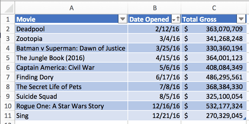
Let’s take a simple worksheet like the following:
You can also copy and paste this data into your Excel workbook to follow along:
| Movie | Date Opened | Total Gross |
|---|---|---|
| Deadpool | 2/12/16 | $363,070,709 |
| Zootopia | 3/4/16 | $341,268,248 |
| Batman v Superman: Dawn of Justice | 3/25/16 | $330,360,194 |
| The Jungle Book (2016) | 4/15/16 | $364,001,123 |
| Captain America: Civil War | 5/6/16 | $408,084,349 |
| Finding Dory | 6/17/16 | $486,295,561 |
| The Secret Life of Pets | 7/8/16 | $368,384,330 |
| Suicide Squad | 8/5/16 | $325,100,054 |
| Rogue One: A Star Wars Story | 12/16/16 | $532,177,324 |
| Sing | 12/21/16 | $270,329,045 |
Now we’d like to find the top grossing films of 2016 and then sum them up to give us a grand total. How do we go about doing that?
Getting the Top 5 Values
First, we need to get the top 5 values from the list. We can do this by using
the LARGE() function in Excel. If you’re not familiar with the LARGE()
function, click here to learn more.
Normally, you would use the LARGE() function to return a single value, but
today, we need it to return multiple values. To do this, select 5 cells and then
in the formula bar type the following formula:
=LARGE(MovieData[Total Gross],{1;2;3;4;5})Then press Ctrl+Shift+Enter to create an array formula.
The formula should look like this in the end:
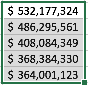
{=LARGE(MovieData[Total Gross],{1;2;3;4;5})}Since you had 5 cells selected, the values will be spread across the 5 cells from top grossing film to least grossing film.
Here are the results of that formula:
OK, we have the top 5 grossing films, now all that’s left to do is sum up those values.
Putting it All Together
In a single cell, you can take that LARGE() function we wrote earlier and wrap
it with the SUM() function:
=SUM(LARGE(MovieData[Total Gross],{1;2;3;4;5}))Be sure to enter this formula with Ctrl+Shift+Enter.
And with that, you end up with the top 5 grossing films:


