Excel Formulas for Beginners
April 26, 2012
Formulas are the basis of getting any calculation done in Excel. Whether you need to sum a range of values, calculate forecast for next quarter’s sales, or even to perform text manipulation, all these things are done using formulas. Simply put, Excel without formulas would just be a fancy text editor (ok, maybe a little more than that, but you get my point). Formulas are a crucial part of being efficient in Excel and if you’re brand new to formulas, this post can be of great use to you.
What are Formulas in Excel?
As mentioned in my An Introduction to Microsoft Excel, Excel uses a grid of cells to contain data. Whether that data is text, numbers, or both, you can apply formulas to it in order to produce useful information. For example, you can sum all of the data in a column, find the difference between two dates, or combine multiple strings together.
How to Write a Formula
Writing a formula in Excel is easy. Here are 3 basic rules to remember before you write a formula:
- A formula always begins with the equal sign (=)
- All built-in functions (like
SUM()) always have parenthesis after the function’s name and after all the arguments have been passed to that function (more on arguments later) - Formulas accept numbers, text, or cell references
You write your formulas by selecting the cell you wish to have the formula’s output be displayed and you can begin by typing the ”=” sign. You can also click inside the formula bar to enter a formula or you can press F2 (which brings your cursor to the formula bar for the selected cell).
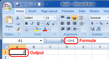
Here is an example of a simple formula:
Notice that the formula bar shows the formula while the cell shows the output. This is because a) the formula bar always shows the formula (hence, its name) and b) I’m currently not in an “Edit Mode” where I could change the formula.
To edit a formula, there are 3 convenient ways you can use:
- Double-click the cell that has the formula (this will temporarily make the cell into a formula bar to edit the formula from within the cell)
- Select the cell and click in the formula bar
- Select the cell and press F2
Cell References
In my previous example, I added two numbers by entering the actual numbers into the formula. What if I needed to grab a number from a cell? That’s easy. You can either type the cell reference by hand, or you can select the cell you want to reference while still editing the formula.
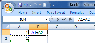
In the following image, notice how A2 has a weird dashed outline to it.
That’s because I recently selected it.
The output will still be 2 as shown previously. Also, did you notice the colors
of the A1 and A2 text? They are blue and green, respectively. Their cells
are also outlined with those colors when you are editing the formula, but it’s
hard to see that in the image because all of the cells are against each other.
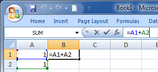
Check out the next image below. This time I clicked in the formula bar to
better see the color outline. This gives you a visual guide to where the
references are made. (Also, since I clicked in the formula bar, the colors are
displayed there rather than inside cell B1.)
It’s important to know that when Excel evaluates a formula, it starts by looking
at the references and converts them into their respective values. So for the
formula above, A1 converts to 1, then Excel converts A2 to 1 as well,
and then it sums them together. When the reference is a range, it is
converted into what’s called an
array,
or a collection of values ordered in the way they were found (left to right,
move one row down, then repeat).
Related articles:
Excel’s Built-In Functions
Excel provides a ton of built-in functions you can use in your formulas. There are formulas for math, finance, statistics, and even engineering. Excel can be very powerful with its built-in functions.
Each function takes in what’s called an argument (or multiple arguments). An argument is some information that the function needs in order to do what you want it to. Usually, when a function takes one argument, the argument is just a reference to the data you want to have the function work on. If there is more than one argument, then some of those arguments are just instructions for the function on how to process the data. Each argument is separated by a comma. Also, arguments can also be called parameters.
For now, we’ll begin with a simple SUM() function. In later posts I’ll be sure
to get more in-depth with other useful functions.
The SUM() Function
The SUM() function does just what it says, sums up data. It requires at least
one argument, but can take up to 255 arguments. Each argument “type” can either
be a cell reference, a cell range reference, or a hand-typed number. The
argument types can be mixed and matched. To follow our simple example of
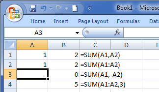
A1+A2, here are some ways you can use the SUM() function.
Allow me to explain how these 4 formulas work:
- Two basic cell references, separated by a comma. So in this formula there are two arguments to the SUM() function. The result is 2.
- The argument here is the cell range. I should mention that you define a cell range as Start:End where Start is the top-left-most cell and End is the bottom-right-most cell. The two references are joined by a colon. The result is also 2.
-
In this formula, I put a reference to
A1, which is 1, and a reference toA2, which is also 1. However, for theA2reference, I also put a dash (or hyphen) in front of the reference. This dash negatesA2'svalue, making it -1. So 1 + (-1) = 0.- Remember that Excel evaluates the reference first, and then applies functions and operators (operators are +, -, *, /, etc.) For example, when it sees
-A2, it first convertsA2to 1, and then negates it.
- Remember that Excel evaluates the reference first, and then applies functions and operators (operators are +, -, *, /, etc.) For example, when it sees
- The fourth formula is just a cell range as the first argument, followed by a hand-typed “3” as the second argument. The result is 1 + 1 + 3 = 5.
What’s Next?
Start writing formulas! The best way to learn Excel is by actually playing around with it. You can start by check out some of the Commonly Used Excel Formulas.
You can also get started with Vlookup, one of the most popular formulas in Excel!


