Vlookup in Excel

July 31, 2012

Vlookup (pronounced ”vee-look-up”) is one of the most popular look up functions in Excel. When you need to extract data from a table based on a particular value, you can use Vlookup to do that. In simple terms, it looks at a table in the first column for a specific value and returns a cell in the same row where you choose the column to return from. You get to choose whether you want to find an approximate match or an exact match (more on which one to choose later). You can use this for both text searches as well as numeric searches, which proves to be a powerful function and can easily help you out in your everyday tasks at work.

What we’ll be talking about:

Vlookup function basics
Vlookup with text searches
Vlookup with numeric searches
When to choose approximate match versus exact match

Let’s get started.

Vlookup Function Basics

The Vlookup function has the form of:

=VLOOKUP(lookup_value, table_array, col_index_num, [range_lookup = TRUE])

Here is a simple explanation of each parameter (for those of you who don’t know, a parameter is, check out this post):

Parameter	Notes
`lookup_value`	The number or text sought for.
`table_array`	A cell reference of the table range. Note: Do NOT include headers in your cell reference if you are searching for text and an approximate match. Trust me, you won’t get the desired results in some cases (more on that later).
`col_index_num`	The number of the column you want to return. This number is based on the table you pass, not by the column character’s number equivalent. For example, if your range is `B2:D5`, column 1 is `B`, column 2 is `C`, and column 3 is `D`.
`range_lookup`	Can either be `TRUE` or `FALSE`. It s an optional parameter where if left out, the value is set to `TRUE`. If `TRUE`, the function will look for an approximate match. This means that for a numerical search, it will return the closest number smaller than the value you’re looking for, if it does not find an exact match. If `FALSE`, the function will look only for an exact match. And if no exact match is found, an `#NA!`error will be returned. I should note that if you choose `TRUE` for `range_lookup`, the first column in the table must be sorted from smallest to largest (or for text, alphabetical).

Does this article help you? If so, please consider supporting me with a coffee ☕️

Vlookup when searching for text

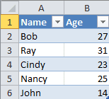
Here I create a simple table to illustrate using Vlookup when searching through text. Let’s say that I want to find the age of someone based on the name we’re searching for.

(If you’re curious as to how I have those little dropdown buttons next to each header name, select your table - including the headers - and click Sort & Filter -> Filter)

Say we want to find Ray’s age using the Vlookup formula. Here’s how we would do it:

=VLOOKUP("Ray",$A$2:$B$6,2,FALSE) Result: 31

Here is the formula breakdown (each parameter is separated by a comma):

Parameter	Notes
`"Ray"`	The text we’re searching for in the first column of the table array we will pass. (Hint: this can be a cell reference instead of just plain text)
`$A$2:$B$6`	The table array. We have to include column `B` because that is what we want to return based on the text we find in `A`.
`2`	This is the column number.
`FALSE`	This tells the function that we want an exact match. A nice thing about using `FALSE` here is that we don’t have to worry about the table being sorted. I’ll get into what happens when we use `TRUE` in a little bit.

When the formula is evaluated by Excel, it looks in each row of column A for an exact match on “Ray” which we passed as the parameter to search for. The formula then finds “Ray” in the second row of the table we passed (remember, the first row/column starts and the top-left-most cell in the table passed to the function). When it finds “Ray” it moves to column 2 in the table of the same row and returns 31, which is correct.

Vlookup when searching for numbers

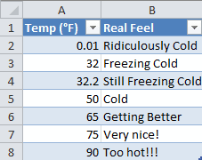
It’s more likely that you’ll search for an approximate match when looking for a number when using Vlookup (or at least that’s what I think, anyway). Check out this basic table showing temperature and corresponding “Real Feel.”

Let’s look at some of the return values by playing around with the Vlookup formula. I’ll do a Vlookup on a temperature of 0.03 using this formula:

=VLOOKUP(0.03,$A$2:$B$8,2,TRUE) Result: "Ridiculously Cold"

Let’s look at the formula breakdown and then we’ll step through how it came to that result:

Parameter	Notes
`0.03`	The number we’re trying to find a close match for.
`$A$2:$B$8`	The table array (again, including column `B` so we can return the “Real Feel”).
`2`	The column number we want to return. In this case, the “Real Feel” value.
`TRUE`	This time we tell the function that we want an approximate match. So when we looked for `0.03`, we found a match for `0.01` in the table. Again, remember that when we set this value to `TRUE` we must have the table sorted and we cannot have the header as part of the table range (I’ll explain why in a little bit).

The way Excel steps through this formula is similar to the last one we looked at:

It starts by looking at the table’s first column for a value of 0.03 or something close (approximate).
Starts with 0.01. Since 0.01 is less than 0.03, it moves to the next one.
Then it looks at 32. Since 32 is greater than 0.03, it reverts back to 0.01 as the closest match.
Now it goes to column 2 and return the corresponding value next to 0.01’s value, which is “Ridiculously Cold.”

If we were to change TRUE to FALSE, we would receive the dreaded #NA! error since there is no 0.03 value in the table. The range_lookup value can be more important than people realize when using Vlookup.

So what if we tried searching for 31 instead of 0.03? Should we have “Freezing Cold” be returned? Let’s take a look.

=VLOOKUP(31,$A$2:$B$8,2,TRUE) Result: "Ridiculously Cold"

What?! It returned “Ridiculously Cold”? But 31 is WAY closer to 32 than it is to 0.01. What gives?

Remember what I said before about the range_lookup parameter for numerical searches?

For a numerical search, it will return the closest number smaller than the value you’re looking for, if it does not find an exact match.

Let’s step through how Excel evaluated this formula:

Is 0.01 less than or equal to 31? Yes, it is less. So keep moving down.
Is 32 less than or equal to 31? No, so we can stop looking.
0.01 is considered the closest approximate match in this scenario, as odd as it may seem.

It’s clear that searching for an approximate value will sometimes seem less logical than we think it should behave. Let’s look at the quirks of Vlookup and see if we can make some sense out of it.

Approximate match or exact? Which one should I choose?

The range_lookup parameter is what controls whether we tell the Vlookup function should look for an exact match or an approximate match. This setting can be a bit tricky so it’s good to remember how the function will be behave based on this value and which one you should choose when using the Vlookup function.

Exact Match

This is just my opinion, but I feel that searching for an exact match makes this function much easier to use. This is especially true when searching for a text value (which I feel is what most people actually use when people use text for the range_lookup parameter). Chances are you would only want to find an exact match when searching for text.

A nice feature of searching for an exact match is that you don’t have to worry about sorting the table by the column you’re searching for. This way, when your table grows, the formula still works correctly.

Also, with exact searches, you can safely include the header row when you pass the table parameter.

Approximate Match

Approximate matches are probably best-suited for numerical searches. Searching for exact matches might be more difficult when your numeric values contain fractions of numbers. I would imagine that in most cases, looking for an exact numeric match would be very difficult when dealing with fractional numbers. I feel that approximate match is more appropriate in this kind of situation.

When searching for text, however, it’s difficult to find a good reason to look for an approximate match. And what would be considered an approximate match, anyway? If we search for “Baub,” would “Bob” be an approximate value? In this case, no. That’s because alphabetically, “Baub” comes before “Bob.”

Yet, there are times where the approximate match doesn’t seem to make the most sense like we saw earlier. I guess it’s in the name “approximate.” When you hear that, you think of what’s closest to what we’re looking for. To help remember how approximate matching works, think of it as “the closest match less than or equal to the value sought for.”

What’s with excluding the header row?

OK, I know I mentioned this a few times in this post. Here’s the thing, when you search for text using approximate match and you include the header row as part of your table, you will not always get the desired results. Let me show you an example. Let’s look at our first table:

This list is sorted by name. Check out this formula:

=VLOOKUP("Bob",$A$1:$B$6,2,TRUE) Result: #NA!

We have the range_lookup value set to TRUE which means to look for an approximate match. Yet we get an error in return. This is really strange, because if we change the formula to this:

=VLOOKUP("Bob",$A:$B,2,TRUE) Result: 27

It doesn’t complain. In my opinion, try to either use FALSE for range_lookup or just don’t include your headers if you have to search for an approximate match.

I hope you enjoyed this post and if you did, please subscribe! You will get notified of newer posts the moment they are published. Also, if you have any questions or comments, or if you want to see me post about something, please leave a comment below. It really helps me to make this blog better and I would love to hear from you.