Use IFERROR() to hide ugly errors
July 10, 2017
Imagine that your boss asks you to create an Excel template for making invoices. You search online for a free template to download and you come across a nice template that can get the job done.

I found this template on Vertex42. If you haven’t checked them out yet, you should. They have a lot of nice free templates and great content on their site overall. Definitely worth a visit.
You start using this for a while and eventually you conclude that it’s very annoying to have to manually type in the items on the invoice for each one you create. You’re looking to be more productive and impress the boss so you decide to add an Excel Table so you can easily reference pricing from that table in your invoice worksheet (the table is named Data).

Yes, this is obviously a contrived table, but you get the point.
You come back to your invoice page and add Data Validation to the Description column so you can use a dropdown to easily select items for the invoice.
Then you add an
Index+Match
function in cell C17 to lookup the price for whatever item you select in the
invoice.
=INDEX(Data[Price],MATCH(A17,Data[Item],0))

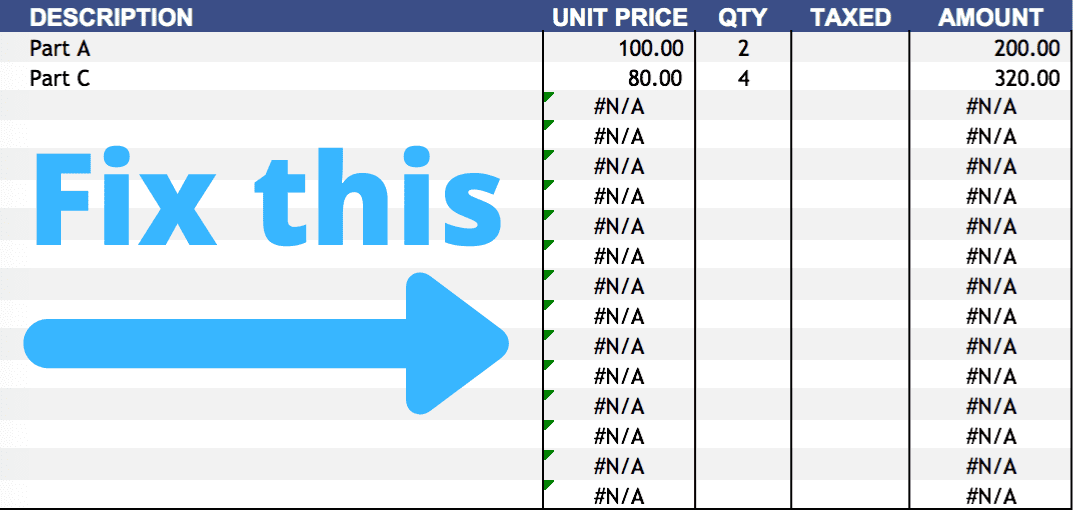
So far, so good. Now let’s copy that formula down through the rest of the Unit Price column.

Yuck. We just ruined a nice-looking spreadsheet. And forget about sending this to a customer - it looks too unprofessional.
Now what do we do?
IFERROR() to the Rescue
Essentially, IFERROR() is a simple way to have your formula do something
specific should an error occur.
For our example, we’ll use the IFERROR() function to hide the errors.
Here’s the IFERROR() function defined:
IFERROR(value, value_if_error)
| Parameter | Description |
|---|---|
value |
This would be your regular formula. In our case, it will be the Index+Match function. |
value_if_error |
This is what you want to do if an error occurs in the value parameter. For our example, we just want to return a blank string "". The types of errors that are recognized by this formula are Formula Error Codes. |
Let’s apply the following formula to fix this issue:
=IFERROR(INDEX(Data[Price],MATCH(A17,Data[Item],0)),"")
Notice all we did here was just wrap our main Index+Match function with the
IFERROR() function. And when an error occurs, we just use the blank string
"".

Looks like we’ve still managed to anger the Amount column…whoops.
No worries, though, we’ll just use the IFERROR() function again!
We’ll update the formula for the Amount column to:
=IFERROR(IF(D17="",1,D17)*C17,0)
Enter this in cell F17 and then copy down.

Voilà. Good as new.
Now the invoice template fully supports having an item lookup through an Excel Table and we have hidden those ugly Excel errors.